Small Angle X-Ray Data – Image Processing
In
this tutorial you will reduce 2D SAXS data to create 1D absolute scaled data.
The data were collected at APS on beam line 15ID on some polymer base materials
to be used for liquid crystal displays. The processing has several steps
including detector calibration (i.e. determine sample-detector distance &
tilt), integration and scaling to an absolute scaled glassy carbon measurement.
The data were collected at a wavelength of 1.0332Å with a MarCCD
detector placed ~570mm from the sample. Note that menu entries are listed in
bold face below as Help/About
GSAS-II, which lists first the name of the menu (here Help) and second the name of the entry in the menu
(here About GSAS-II).
If you have not done so already, start GSAS-II.
Step 1: Detector calibration
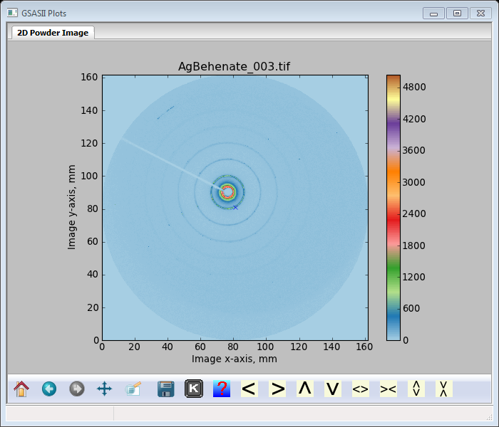
The detector position is determined by using an image collected from silver behenate; do Data/Read Image data… and a file selection dialog box will appear. Go to SAimages/data and select AgBehenate_003.tif with either a mouse button double click or Open; the image will appear
And the Image controls window will show (you may have to select the IMG tree entry & then it’s Image Controls).
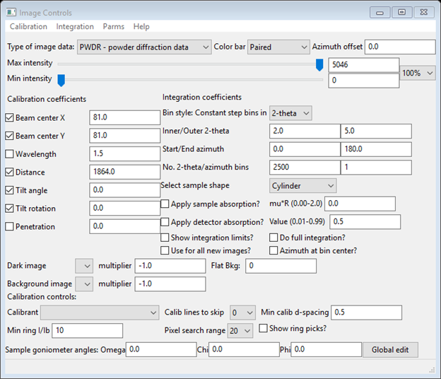
Note the default Type of image data is PWDR - powder diffraction data; you will change that now. Select SASD – small angle scattering data (the window will change). Enter the wavelength (1.0332), and select the Calibrant (near bottom of window) as Ag behenate. Note that the calibration info for Ag behenate was read from a python file – GSASII/ImageCalibrants.py. If you have a calibrant that isn’t in this file you should enter it in the file UserCalibrants.py; just follow the format of the examples within ImageCalibrants.py. You should move the Max intensity slider to near the middle of the range – that will improve the image. When done the Image controls window should look like
And the image will be
![]()
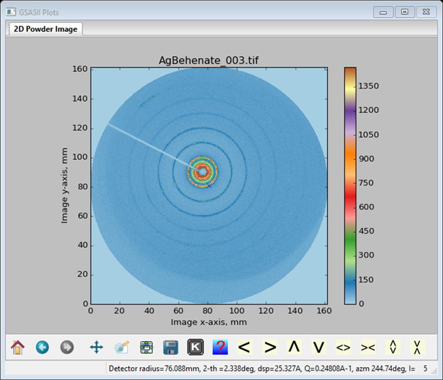
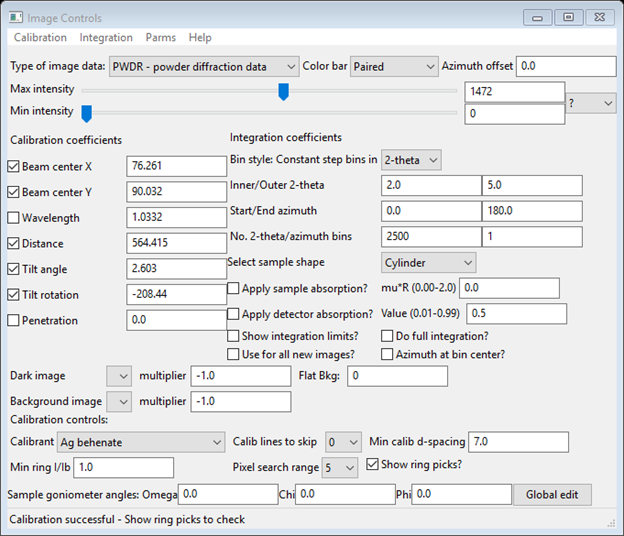
Next select Calibration/Calibrate from the Image Controls menu; a bit of instruction will appear on the status line of this window. Select 5 points on the innermost ring (arrowed above); a small red cross will appear at each selection point. Press the right mouse button to finish; calibration will proceed. A sequence of concentric red rings will appear; they will switch to blue when calibration is finished. Select Show ring picks (near bottom right of Image Controls window). The Image Controls window will show the results of the calibration
And the plot will show the points used in the calibration calculations.

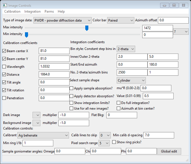
You would like to use more points from just the visible rings. I suggest you change Min ring I/Ib to 0.5 and Min calib d-spacing to 10.0. Do Calibrate/Recalibrate; more points will be used and they will be limited to the 5 visible rings in the pattern.

And give the calibration result as

You will need this calibration information to process the other images in this tutorial. To save it for future use do Parms/Save controls; a file dialog will appear. Makeup a file name (no extension needed) for this; I chose SASD. Press Save and the file SASD.imctrl will be written to the local directory. If you are continuing on to the next step do File/New Project (don’t bother saving the project file unless you want it; we will not need it here); otherwise you can exit GSAS-II.
Step 2: Data image integration
The objective here is to read in the four polymer sample images, a glassy carbon image, an empty container image and a dark image. The images will be integrated after creating masks to remove the beam stop and other objectionable parts of the images. If you have not done so already, start GSAS-II.
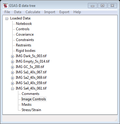
First do Data/Read image data…, go to exercises/SAimages and select all images except AgBehenate_003.tif; then press Open to read all of them. The GSAS-II data tree window will show entries for 7 images and will expand the last one
Notice that the Dark, Empty and GC (glassy carbon) are all 5s images and the Sa1-4 ones are 40s images; this time information is needed later to obtain correct scaling. First select the IMG GC_5s_200.tif entry from the tree and expand it (press the + box); then select Image controls. The data window (Image Controls) will show the default settings.
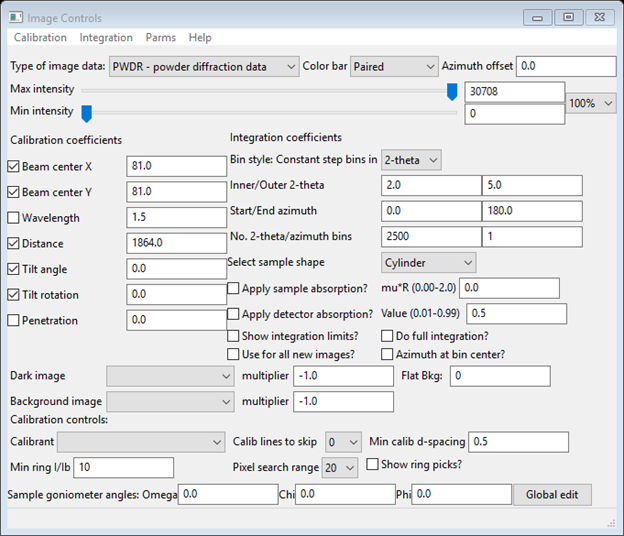
Do Parms/Load controls from the menu; a file selection dialog will appear showing the available *.imctrl files (the one you made in Step 1 should be seen). Select it and press Open; the Image Controls window will be redrawn with the settings obtained in Step 1: Detector calibration
and the image will be that of glassy carbon. Changing the Max intensity slider on the Image Controls window will show that the image from the MarCCD is circular and slightly offset from the beam center. You can also select from the drop down to the left of the intensity sliders; 90% will suffice. A beam stop shadow is evident as well as an arc-like fault in the image (a bit hard to see - toward the upper left corner of the image). We will sort those out later.
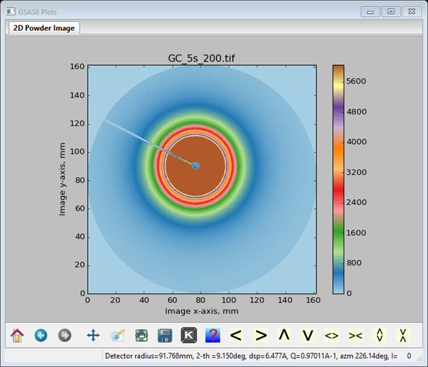
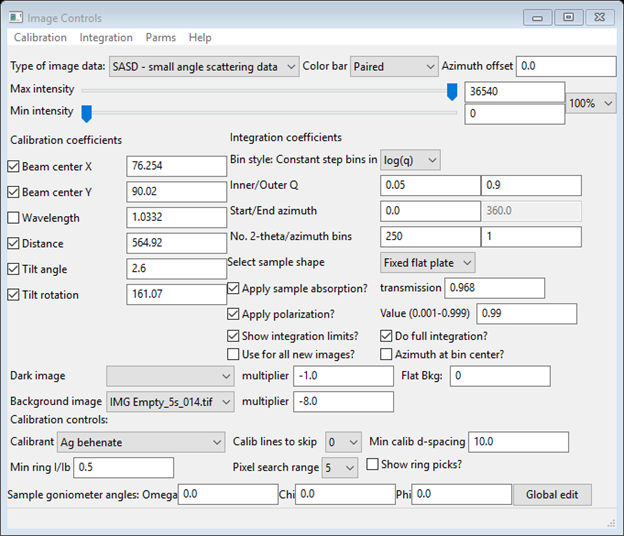
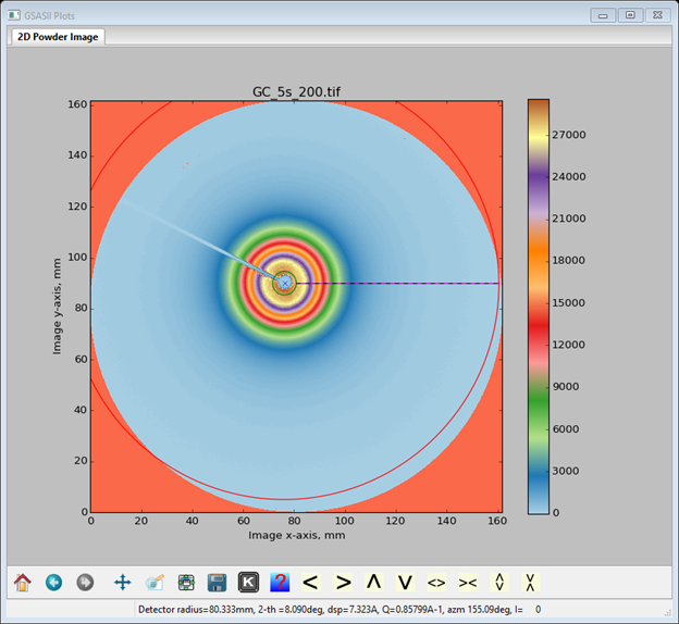
The next step we will be doing is to set up the integration controls. The Dark image is IMG Dark_5s_003.tif, the Background image is IMG Empty_5s_014.tif. We will be needing the background image; the dark is not needed as it would be subtracted from both sample and background thus cancelling out. Select just IMG Empty_5s_014.tif for the Background image; leave Dark image blank. The multiplier is -1.0 because its exposure was the same as this glassy carbon image (5s). Notice that the background is instantly applied to the image. Next check the boxes for Show integration limits? and Do full integration? A pair of circles with a connecting diagonal line will appear on the plot. Set the Inner/Outer q values to 0.05 and 0.9, respectively, and set the Start azimuth to 0. Set the No. 2-theta bins to 250, which is more appropriate for small angle scattering, and set the Bin style: Constant step bins in to log(q). You should also check the Apply sample absorption? and Apply polarization? boxes; set the sample shape to Fixed flat plate and enter the measured transmission (0.818) for the glassy carbon sample. When done the Image Controls data window should look like

And the plot should look like

Now copy these controls to the other images. Do Parms/Copy controls and select just the Sa1-4 data names.
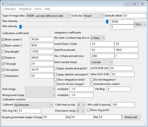
We now need to go to the Image Controls for each of Sa1-Sa4 to enter the correct transmission for each and change the Background multiplier to account for the different exposure times. Start with IMG Sa1_40s_067.tif and change transmission to 0.943 and the multiplier to -8.0. Then go to IMG Sa2_40s_069.tif and change transmission to 0.979; multiplier to -8.0. Next go to IMG Sa3_40s_059.tif and change transmission to 0.960; multiplier to -8.0. Finally, go to IMG Sa4_40s_061.tif and change transmission to 0.968; multiplier to -8.0. The Image Controls data window for this should look like
You will notice that the image changes as you change the Background image multiplier; it applies this correction immediately. Pretty clearly much of the Sa1-4 images are largely background (intensities ~0; negative ones shown as red); we’ll see the result of this when we integrate them.
This is a reasonable time to save the project; do File/Save project as… from the main GSAS-II data tree menu. Choose a file name (I assumed image) and it will be written on the local file directory.
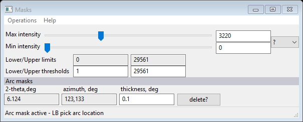
As noted earlier, the images contain some unwanted features; so let’s create masks to remove them. Select Masks from the GSAS-II data tree under IMG GC_5s_200.tif; the data window will show
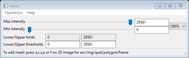
To mask out the regions beyond the circular MarCCD image change the Lower threshhold from 0 to 1; the image will be redrawn with these regions in red
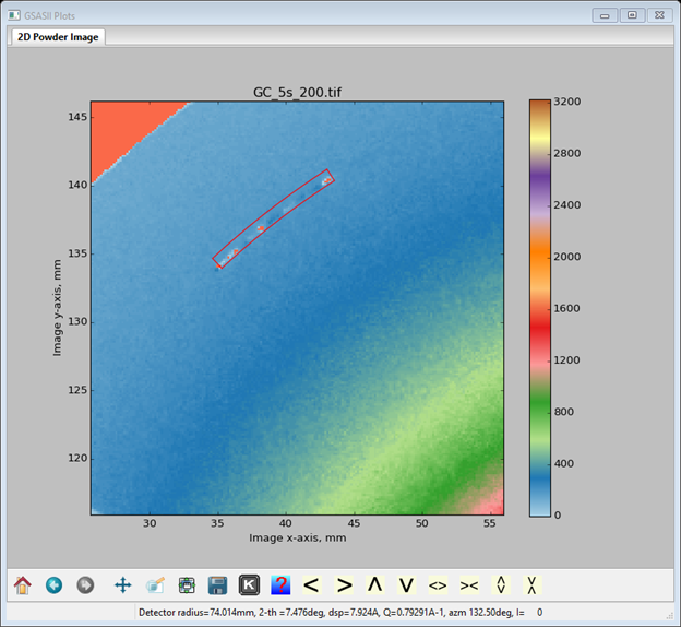
These are now excluded. The status line for the Masks data window gives the directions for adding additional masks. You can make arcs (we’ll use that here), rings, spots (this too) and polygons (this as well) as masks. These enclose areas to be excluded. The frame works in the opposite sense in that everything outside the frame is excluded (NB: only one frame is allowed). So let’s first mask the bad arc in the upper left – zoom in on that part of the image

To add the mask 1: be sure the focus is on the image and the zoom buttons are off, 2: type a to activate the arc mask entry 3: press the left mouse button (LB) with the cursor centered on the bad arc. The Masks window will show a new entry
and an arc mask will be drawn on the plot.
You can change the angular width of the arc by changing thickness in the Masks data window, you can change the angular range of the arc by RB dragging either end of the arc (NB: increments only in whole degrees), and you can move the arc along a constant 2Θ angle by LB dragging on any edge of the mask. The curvature is centered on the beam center position and follows a constant 2Θ curve established by the detector calibration.

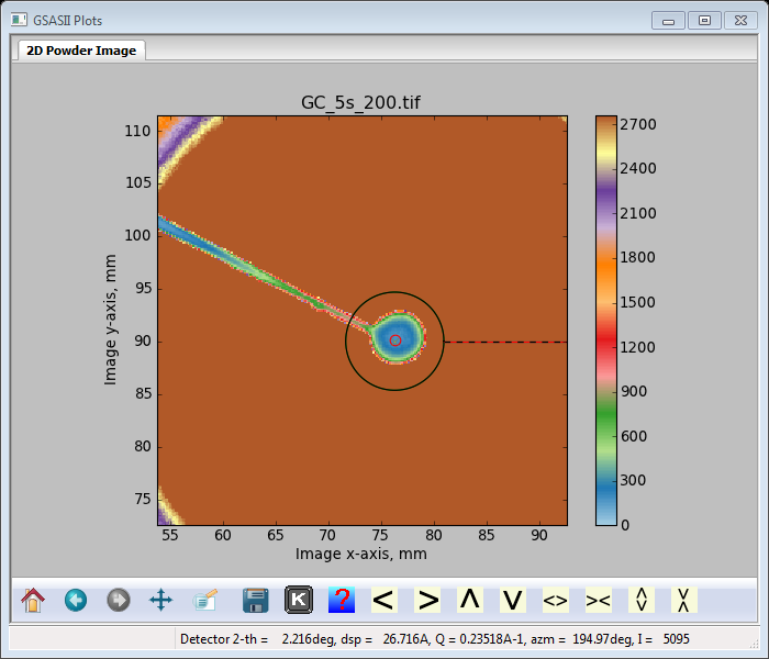
Next let’s deal with the beam stop. I’m going to use both a polygon and a spot to cover it. Move the zoom area to be around the center, make sure the zoom buttons are off, enter ‘s’ on the plot and press mouse LB with the cursor positioned where you want the spot (probably on the ‘X’ – beam center position). A 1mm diameter red circle will appear on the plot
And the Masks window will have new information
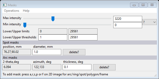
You can change the diameter of the spot, I used 7.0; the plot now shows a ring that just covers the beam stop. You may have to drag it a bit (Hint: drag the center of the spot) to get it well centered.

Next we need to mask the stick holding the beam stop; we’ll use a 4 sided polygon for this. Adjust the zoom & position so you can see the entire beam stop stick. Make sure all zoom buttons are off, press ‘p’ on the plot, then press the mouse LB at four points in succession around the beam stop stick. A line segment for the polygon will be drawn following your mouse clicks. Finally press the mouse RB to close the polygon. You should see something like

You can adjust the position of the polygon vertices by closely dragging it with mouse LB pressed; a new vertex can be added by dragging an existing vertex with the mouse RB pressed. If you drag one vertex onto another, they are merged and cannot be separated.
We want to use these masks for all the Sa1-4 images. Do Operations/Copy mask; a Copy mask information dialog box will appear. Select the Sa1-4 items and press Ok. Here is a useful place to save your project; do File/Save project from the main GSAS-II data tree menu.
Step 3: Integration of images
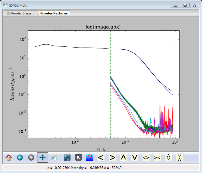
We are now ready to integrate the glassy carbon and the four Sa images. Select any Image Controls and then do Integration/Integrate all. A selection dialog will appear; select only the GC and Sa1-Sa4 data sets and press Ok. The image integration will proceed; a progress bar increments as each one is done. Five SASD data items will appear on the GSAS-II data tree; the last one (SASD Sa4_40s_061.tif Azm=0.00) will be expanded and plotted (you may have to select the Powder Patterns tab to see it).
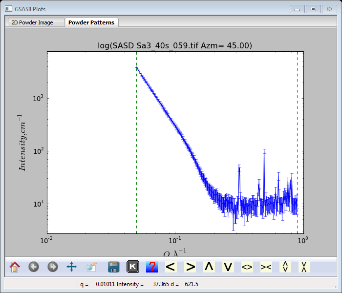
Pretty obviously the SASD pattern is down to background at Q~0.25Å-1; the other Sa1-Sa4 patterns are similar. The glassy carbon pattern extends nicely to the highest Q (~1.0Å-1) measured.

Step 4: Scaling of SASD patterns
To set this data on an absolute scale, we compare it to an absolute scaled glassy carbon scan. One of these is in the same directory as the image data; do Import/Small Angle Data/ from q(A-1) step X-ray QIE data file and select GC calibrated data.txt from the file selection dialog. You will need to select any file(*.*) to see it. A Is this the file you want dialog will appear – respond Yes to read the file; it will be plotted.

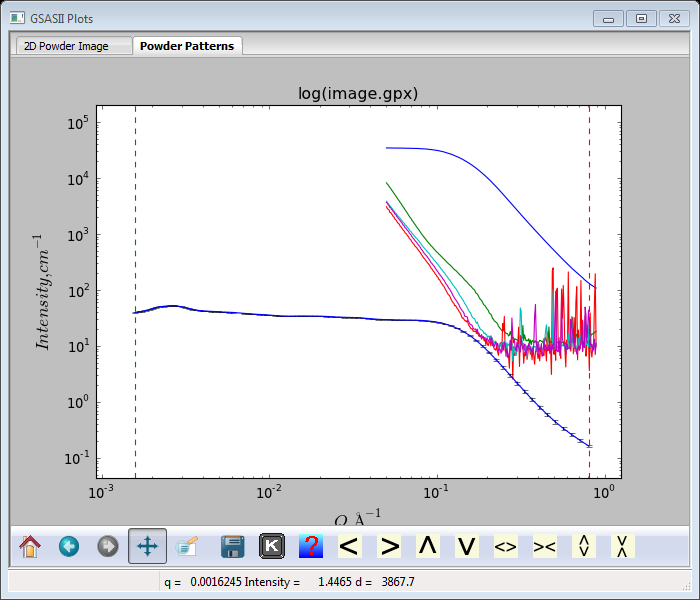
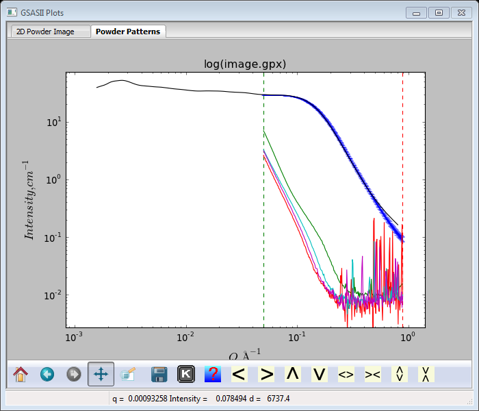
If you enter ‘m’ on the plot window, all of the SASD patterns will be plotted together (I’ve adjusted the zoom to see them all).
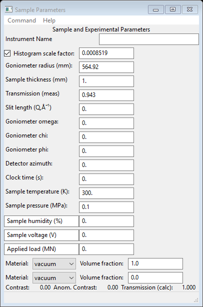
Clearly the measured image data need to be scaled down to have them on absolute scale. First is to discover the scaling between the two glassy carbon patterns. Go to the measured one (SASD GC_5s_200.tif Azm=0.00) and select Sample Parameters.

We will change Histogram scale factor by comparison with the absolute glassy carbon scan. Do Command/Set scale from the Sample Parameters menu; a Reference histogram dialog will appear.
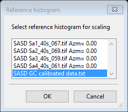
Select SASD GC calibrated data.txt (shown in blue above) and press Ok; the GC_5s_200.tif data will be rescaled to the GC calibrated data and the Histogram scale factor will be changed to the new scaling factor (0.0008519). The plot will be redrawn with the scaled data.
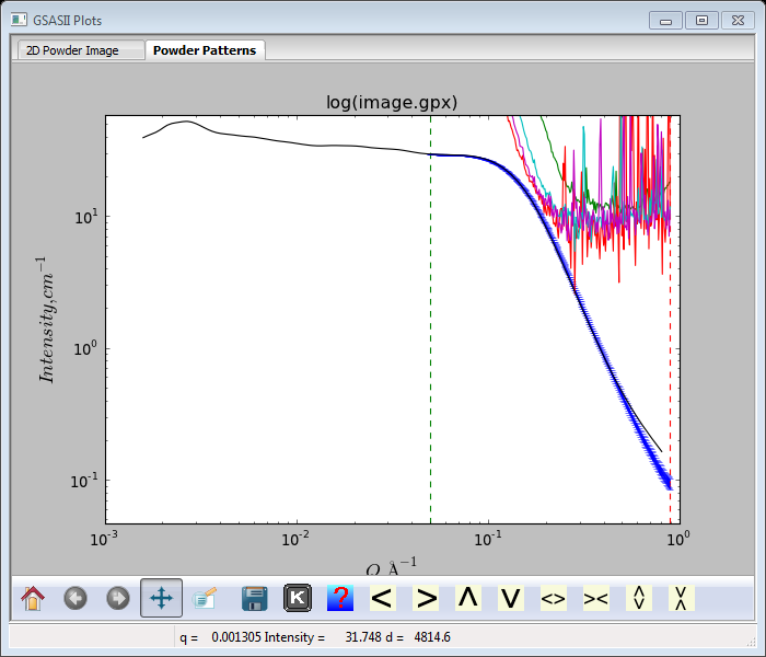
The divergence at high Q is probably from a background contribution to the standard that is not present in our measured one. Next we have to apply this scale factor to the Sa1-Sa4 data sets. Do Command/Copy selected… from the Sample Parameters menu; a Select sample parameters dialog will appear
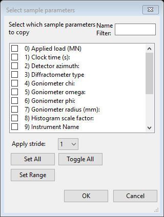
Select only Histogram scale factor (#8) and press Ok; a Copy sample parameters dialog will appear
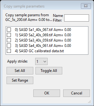
Select only the Sa1-Sa4 data sets and press Ok. The copy will occur and the plot redrawn
I’ve changed the zoom to show all the data. We are not quite done; the scales for the Sa1-Sa4 data sets have to be further reduced by a factor of 8 to account for the longer exposure time. Select SASD Sa1_40s_067.tif from the GSAS-II data tree, expand it and choose Sample Parameters
The data items here can take simple mathematical expressions so change Histogram scale factor to 0.0008519/8 and press Enter. The value will change to 0.0001065 and the plot redrawn.
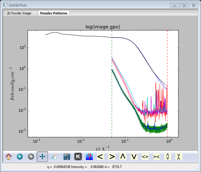
Next do Command/Copy selected as before to copy this new scale factor to the other Sa data sets. The plot will again be redrawn
Everything is now on absolute scale and these polymer samples are quite weak small angle scatterers. This is a good point to do a File/Save project from the main GSAS-II data tree menu. You can try to fit unified & Porod models to them following the procedures demonstrated in the Fitting Small Angle X-Ray Data tutorial. I’d set the high Q limit to about 0.25Å-1 as above that is only noisy background.